In my previous Loop Signatures article (see www.instrumentation.co.za/16775r), the purpose of the derivative (D) term and the two types of processes where it works effectively were discussed. This article and the next will deal with the practicalities of using the derivative as applied in the modern digital controller.
As was demonstrated, if a ‘vertically’ changing input signal (like a step change) is applied to a derivative block, the block’s output (in theory) should go to infinity. An example of this is shown in Figure 1, where a P+D controller in the test rig is subjected to a step change in setpoint. The PD (controller output) immediately spikes up to maximum, and then comes straight back down again.
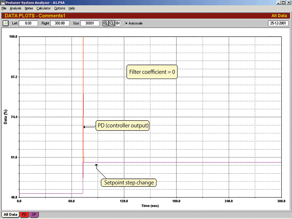 Figure 1. Example of a P+D controller in a test rig which is subjected to a step change in setpoint.
In the old analog electronic and pneumatic controllers, a response like this was impossible as their speed of response was limited by natural lags inherent in the way they worked; examples being the speed of pneumatic signal propagation and capacitor charging time. However, in a digital system that uses mathematical calculations, the maximum output value would be limited only by the number of bits used by the system.
Furthermore, as a digital system is non-continuous and operates on a scan rate, even the smallest change from the previous scan would be seen as a step and the output would go to a maximum or minimum limit. Therefore, a digital system using a straight derivative block would be unusable, as the output would be continually jumping up and down between limits.
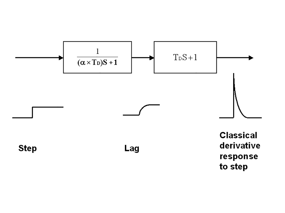
Manufacturers studied the derivative action of the analog units and inserted a first-order lag filter in front of the derivative block, to make their digital controllers operate in a similar fashion. This is illustrated in Figure 2. The filter acts the same way as the natural lags do in an analog system. A step change is now converted into an exponential lag response, and the derivative of this is the classical derivative response.
It is necessary to discuss the strange whims and peculiarities of some of the manufacturers. As mentioned in previous articles, there are no standards whatsoever in the control field, and particularly so when it comes to controllers. The manufacturers not only make their brands of controllers uniquely different to other brands, but many of them may not even make the next batch of controllers, or next version of controller software, the same way.
So, any software version or a different model of controller coming out of the same stable may be completely different – which is obviously highly confusing to the user. For example, some manufacturers do not place the derivative filter before the derivative unit, but before all three blocks (P, I and D). In other words, they put a filter in front of the whole controller. There seems to be no logical explanation for this, as it also affects the tuning of the P and I terms.
The most confusing thing when it comes to the derivative filter is how individual manufacturers handle its value. As can be seen in Figure 2, most controllers have the time constant of the filter set to a value given by:
TC = α x TD, where α is a constant and TD is the derivative time.
This is done to effectively make the derivative response directly proportional to the value of the derivative time, TD. If it was not done this way, then it would be necessary to change the filter time constant every time TD was changed.
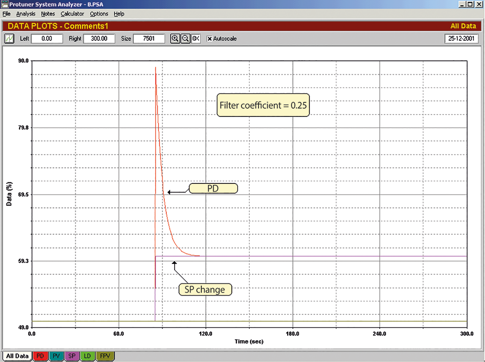
The value of α is especially critical. Most manufacturers set its value to somewhere between 0,125 and 0,25, and generally don’t let the user adjust it. The response of a P+D controller with a derivative filter α coefficient of 0,25, to an input step change in error, is shown in Figure 3. This is a typical classical derivative response to a step change.
In my previous Loop Signatures article, I wrote about a senior instrument technician in a paper plant who believed in using the derivative in every loop. On examining his DCS system (which is a very popular and well-known make), it was found that the value of the α coefficient was user-adjustable, and had been set to unity. To understand the effect of this, it is necessary to look at the combined transfer function of the filter and derivative block. This may be written as:
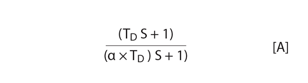
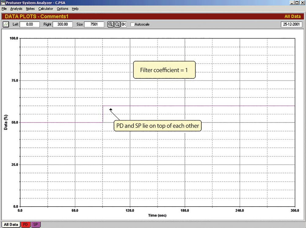
If we set α = 1, then the equation becomes:

Thus, the filter cancels out the derivative term. Figure 4 is the response of the same P+D controller to an input step change in error, but with the α coefficient of the derivative filter set equal to unity. The derivative kick is entirely gone, and all that is left is a purely proportional response.
The senior technician was very embarrassed when this was explained to him. His men had spent months tuning derivatives into loops without realising that the derivative was in fact not working at all. However, it was not altogether his fault – nobody had ever taught him about a derivative filter.
Reference to the DCS user’s manual showed that unity is the default value set by the manufacturer. The manual indicated that the α coefficient was adjustable anywhere between 0,1 and a 100. There was no other reference in the manual to this coefficient, and the instrument technicians in the plant said that in their training courses on the DCS, no mention had ever been made of it. Why would a manufacturer set a default value in the system that effectively switches one of the parameters off? It is completely senseless.
Taking this further, I was recently working in a large South African petrochemical refinery where another well-known make of DCS was installed. Upon finding a temperature loop where D would be beneficial, the manual was consulted to determine the α coefficient. It was found that the coefficient was adjustable over a wide range, but in this case the manufacturer’s default value was 2,5. This is amazing, as it makes the denominator in Equation A larger than the numerator.
The former is a lag, and the latter (D component) is a lead. When you have a lead divided by a lag, and the lead is smaller than the lag, the expression turns into a lag. In other words, the D parameter with its filter is now acting as a large lag on the controller output. The effect of this is shown in Figure 5 on the same controller with the α coefficient set to 2,5. It can be seen that the controller now takes over three minutes to respond to a 10% change in error!
 Figure 5. Effect of having a lead divided by a lag, when the lead is smaller than the lag.
It is hard to believe that a leading manufacturer of control equipment can put such a stupid value of the α coefficient into its controller as the default value. In the company’s particular manual it does talk about the α coefficient and says that it is adjustable, and that a larger value should be used in the presence of large noise on the PV signal.
This is really not a sensible approach; the D term was never intended to act as a noise filter. If one has to attenuate noise, then the DCS has a proper lag filter which can be placed in front of the incoming PV signal. (Please refer to other articles on the dangers inherent in using large filters). One can only conclude that some of the manufacturers, or at any rate, the people writing their controller software, have no real understanding of the practicalities of control.
It is of interest that the people who had commissioned the refinery had brought in an expert on refinery control from overseas to tune the controllers. He obviously also had no idea of the practical aspects of the α coefficient, and had increased the P gain dramatically to overcome the tremendously sluggish response when he used the D term.
About Michael Brown

Michael Brown is a specialist in control loop optimisation, with many years of experience in process control instrumentation. His main activities are consulting and teaching practical control loop analysis and optimisation. He now presents courses and performs optimisation over the internet.
His work has taken him to plants all over South Africa and also to other countries. He can be contacted at: Michael Brown Control Engineering CC,
| Email: | [email protected] |
| www: | www.controlloop.co.za |
| Articles: | More information and articles about Michael Brown Control Engineering |


© Technews Publishing (Pty) Ltd | All Rights Reserved
 printer friendly version