A week before writing this article I was giving a course at a remote mine in the middle of the Namibian desert. We were discussing tuning responses, and as I always do on my courses, I mentioned that, in my opinion, a ¼ amplitude damped tuning is not desirable and is in fact not good.
One of the delegates who recently was awarded with an instrumentation and control technician qualification took exception to this. He said that every book he has read on the subject and all tuning courses say that ¼ amplitude damping is the ideal tuning. He asked who I think I am to go against what everyone else says is right. He went on to say that if he had tuned loops in his trade test, or answered a question on tuning that did not use ¼ amplitude damping, he would have failed.
This is a problem. Unfortunately, at the risk of causing some offence, I have found that many teachers of control have little knowledge of the practical side of the subject, particularly when it comes to optimisation of regulatory control systems. My reasons for not liking ¼ amplitude damped tuning were listed in Loop Signature No. 24 and are as I believe, solid. There is no doubt in my mind whatsoever that such a tune is not suitable for practical control. Apart from this, each and every loop requires its own special tuning and this article will list every possible consideration I can think of which should be taken into account when deciding on tuning.
The different requirements that may have to be taken into account when tuning a process include:
Knowledge of the control system: Loop signature articles 9 through to 16 illustrate the need for a control practitioner to have an in-depth understanding of the control system, features and choices if he wishes to successfully optimise the plant. Good examples of this are the need to trigger control blocks correctly, scaling controller input signals correctly and understanding the differences between PID, PI-D and I-PD responses on setpoint changes.
Possibly one of the chief causes of loss of potential profits in a plant is due to poor controller setup, usually due to an entire lack of knowledge of the features and options available in the system. I have previously cited many examples of plants losing money like this, including a pharmaceutical company in the UK which could have produced millions of pounds of additional products in its batch reactor plant if they had only used the correct controller response to setpoint change.
Tuning for steady state tracking: The purpose of the vast majority of the controllers in continuous process plants (which are running in steady state condition for most of the time) is to minimise variance throughout all stages of the process. This means that the controllers must keep processes as close to setpoint as possible at all times, particularly through periods when load disturbances are occurring. A good example of this is day-night temperature variations.
To accomplish this it is necessary to use a fast tune with an integral as fast as practically possible. The integral is the tuning term that does the most to eliminate control error. Pole cancellation tuning does much to achieve this – see later. It is also essential in achieving this control objective that cycling due to valves or other problems be eliminated.
Good response to setpoint changes: A few years ago, it wasn’t uncommon in plants to find many loops where the setpoint was changed frequently. There were exceptions to this, such as secondary controllers in cascade systems or ratio control. However, today many plants have implemented advanced control systems or are in the process of doing so. Advanced control systems normally set the setpoints of the base layer, (regulatory controllers). It can only be effective if the base layer controllers follow setpoints really well with minimum variance.
Theoretically, a ¼ wave damped tuning is the best tuning for this as it keeps variance to a minimum. However, in the articles referenced above, it was shown that such tuning is not practical or indeed desirable. In practice, we find that tuning with a gain margin of about 6 d.b, which is about 25% slower than ¼ wave damping works well. Such a tuning does result in an overshoot and an undershoot on self-regulating processes. One should check that this is acceptable as overshoots are not desirable on some processes.
In addition, it is essential that the controller be set to follow setpoint with preferably a full PID response on error. If you are in the unfortunate position to have a system where this is not available, then at least ensure the response is set to at least a PI-D response on error. If it is left on I-PD response on error, a poor variance will result, particularly on slow processes.
Tuning for load disturbances: It is often necessary to take the effect of disturbances into account when considering the tuning needed in any particular control loop. There are various types of disturbances which may need differing treatment.
Upstream load disturbances: Upstream load disturbances are those that generally occur ahead of the process and can often affect it very adversely. A good example of such a disturbance is found in a heat exchanger where the flow of process fluid through the exchanger changes. Another such disturbance which would adversely affect similar slow loops (such as temperature processes) would be if the pressure of say the heating steam suddenly changes, which could happen if another machine was switched on and also drew steam out the steam header. The feedback temperature controller is tuned to deal with a slow process and can only respond slowly to changes. It was shown in previous articles on tuning in this series that the integral on a self-regulating process is normally set equal to the dominant time constant of the process, which can be quite large on temperature processes.
The disturbance itself may be quite fast, but if it comes into the process from upstream it is normally ‘filtered’ by the actual process lags, and therefore the actual process variable changes very slowly. The feedback control having such a slow integral can only respond to these changes very slowly, so large deviations from setpoint can result, hence increasing control variance.
Ideally, one would like to tune the controller as fast as possible to try and minimise the variance, but even this is often not good enough. In many cases the only real way to properly eliminate variance with upstream load disturbances is to use feedforward techniques. This will be dealt with in a future article in this series.
Downstream load disturbances: Downstream load disturbances are normally caused by the actual control loop we are working on. Typically as shown in previous articles, integrating processes, in particular levels, are often tuned with relatively high proportional gains. This can result in the valve moving sharply in response to setpoint changes or to fast upstream load disturbances. As a result the flow through the valve can change suddenly and by quite large amounts. This may upset other processes downstream.
Minimising the effects on these downstream processes will require different strategies. Typically, very slow tuning may be needed or else a completely different type of strategy, such as non-linear control. Strategies such as these will be dealt with in a future Loop Signature article under the heading ‘Surge and Averaging Level Control.
Cyclic or periodic disturbances: As described in Loop Signature 22, feedback control is no good at all in dealing with these types of disturbances unless they are very much slower than the ultimate period (UP) of the loop. In fact, trying to tune the loop faster, which is something people are always trying to do, actually makes matters worse.
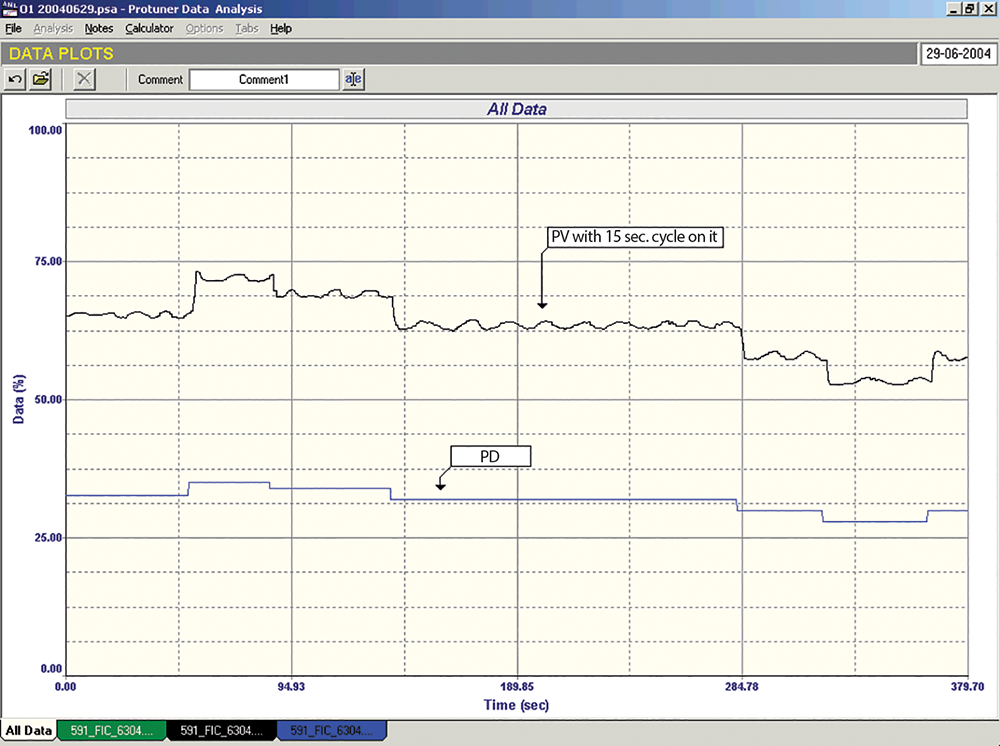
To illustrate this point, Figure 1 shows an open loop test on a flow loop performed very recently at a large chemical plant. The flow has a 15 second cycle in it caused apparently by a reciprocating pump. The plant personnel were trying to tune the flow controller fast enough to catch the cycle. It was determined from the frequency plot obtained from the Protuner that the ultimate period of the flow loop was 5 seconds. Now, as shown in Loop Signature 22, cyclical disturbances coming into a control loop with a period roughly between about 0,2 and 6 times the loop’s ultimate period will cause the variance to increase. The cycle coming into this loop was at 15 seconds, which is 3 x UP, so one would expect the loop to react badly to it.
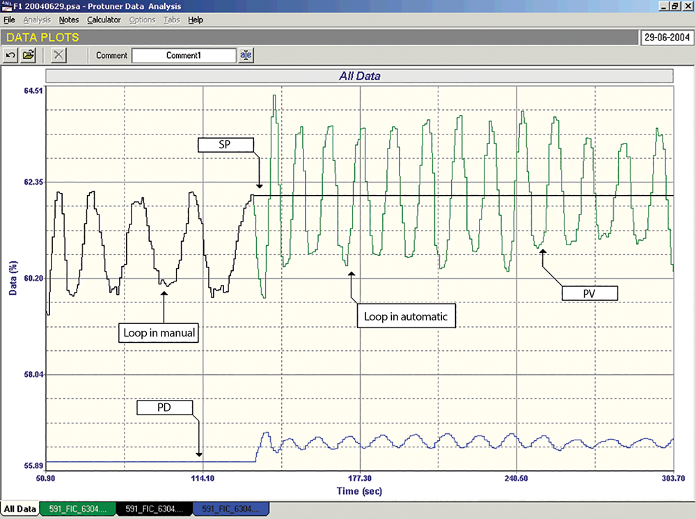
This is in fact what occurred and is shown in Figure 2 where one can see how the variance increased when the loop was put into automatic. There is nothing one can do with feedback control to eliminate this type of problem. If possible, one should try and eliminate the cycle at its source. On certain occasions it may also be possible to use feedforward to cancel out the effects of the cycle on a loop.
Signal noise rejection:
Another factor that can influence the decision on the tuning to use for a particular process is the noise on the PV. This will pass through the controller’s gain amplifier (P term) and will appear on the output of the controller (PD). If high gain is used (such as in level controls) it can present a problem as the valve can start moving around.
In some cases where it is not possible to reduce the noise at the source it may become necessary to use a filter, or else to try and reduce the controller gain to minimise the effects of the noise on the PD.
Just out of interest, the best type of tuning known as ‘pole cancellation’, which should always be used if possible, has the added advantage of giving the lowest gain and fastest integral. Lowest controller gain is good from the point of view of signal noise rejection, and fastest integral gives the quickest recovery from load changes.
Tuning for speed of response versus robustness
In many cases (but not in all), the main requirement of the control is for high sensitivity to process changes such as steady state tracking – see above, where one is trying to keep variance to a minimum. Fast control is needed for this. However, the faster one tunes the controller, the closer one gets to instability. Therefore, you have to balance the speed versus safety. This safety factor is often referred to as robustness.
To do this requires knowledge of the process, understanding what changes may occur under differing conditions and time and of course the control requirements.
This is usually the most important consideration of all.
Process identification
Another absolutely vital consideration is identifying the class and dynamics of each and every process that one tunes. Not only must you know if the process is self-regulating or integrating, but also the dynamic response elements. In earlier articles in this series, process gain, dead time and first order lags were discussed. Future articles will also be looking at all the other dynamics that could be encountered in industrial process control. Certain types of dynamics require very special tuning which can in some instances literally reduce the response time by a factor of four. Even if you use world leading tuning aids like the Protuner, you need the knowledge of the dynamics to achieve the best results.
In conclusion, one can see that there is no such thing as a general optimum tune. As previously discussed, most control teachings postulate that you should always tune with a quarter wave response, which for reasons previously listed, we do not feel is desirable or practical. Instead, one must take into account many, if not most of the various things listed above, before finally deciding how to tune any particular control loop.
In addition, it is essential to work with the process experts and operating staff in deciding on the tuning. Teamwork will also engender cooperation and enthusiasm for optimisation and improvement, and will go far in breaking down parochial attitudes.

About Michael Brown
Michael Brown is a specialist in control loop optimisation, with many years of experience in process control instrumentation. His main activities are consulting and teaching practical control loop analysis and optimisation. He now presents courses and performs optimisation over the internet. His work has taken him to plants all over South Africa and also to other countries. He can be contacted at: Michael Brown Control Engineering CC,
| Email: | [email protected] |
| www: | www.controlloop.co.za |
| Articles: | More information and articles about Michael Brown Control Engineering |


© Technews Publishing (Pty) Ltd | All Rights Reserved
 printer friendly version