

During in-plant courses on practical process control the most interesting part of the course is always the last few days which are spent optimising live loops in the actual plant. Even with a powerful simulator, playing with loops in the classroom is always unreal, and certainly the more experienced and 'battle hardened' control practitioners are always suspicious of 'theory' and slick demonstrations. Therefore there is much excitement when we go out into the field and show how the things we teach actually do apply to real valves and processes. This is where it is possible to demonstrate truly scientific tuning to both the I&C people and to the process people, whom we urge to take part in the training. (Optimisation is a multi-discipline discipline. You must have active participation of personnel from I&C, process and operational staff).
In a recent course in a large chemical processing plant in South Africa, it was decided for the practical part of the training to optimise all the major loops on a particular unit in the plant. This was performed over a three-day period and proved highly successful. Approximately 15 loops were optimised. The performance of 14 of these loops was dramatically improved, with typical response times to load or setpoint changes being between six and 40 times faster. Only one loop remained a problem. This was a bottom level control on a distillation column with a very strange response which exhibited a large negative lead and which was often subjected to fast load disturbances.
A negative lead on a level is a well-known phenomenon on boiler drum level control ('the shrink and swell effect'), but it is unusual to find it on a distillation column. When the controller output was stepped down by 10%, one would expect the level to start rising. However, as can be seen in Figure 1,
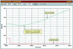
The level first dropped considerably, before starting to ramp up. In all it took approximately 15 minutes before it actually got back to the original level where it was before the step was made.
Unfortunately, feedback control is not good at dealing with such a phenomenon, and one has to treat the negative part of the response as dead-time in the tuning. As has been mentioned in previous articles, the only way of dealing with long process dead-time on a normal PID controller is to detune the controller accordingly. In a case like this, a controller detuned to cope with 15 minutes of dead-time is not capable of catching fast and often frequent load changes. The plant is now investigating the control strategy to try and find some alternative method of controlling this level. If one can measure the load changes, then a good method will be feedforward control.
Another loop that displayed an interesting response is shown in the open loop test in Figure 2.
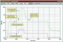
This is a gas flow where the response in the positive direction of valve opening was far faster than in the opposite direction. A response with poor 'mirror image' can be found on certain processes like temperature, but is unusual in flow. The more likely cause here is that there was a problem with the valve. An examination at the valve in the field proved that that this was indeed the case. The valve had an air-to-close response and opened quickly under the return spring action. However, it moved slowly when moving in the reverse direction under air pressure. It was established that the cause of this was insufficient air pressure from the air pressure regulator feeding the positioner.
This was quickly rectified and the vastly improved response can be seen in Figure 3.
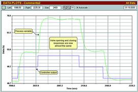
It can also be seen from the figure that the valve is very oversized, as the step change in process variable resulting from a step change in controller output is about four times larger than the latter. (See remarks on process gain below).
Another unusual loop shown in the open loop test illustrated in Figure 4.
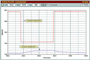
The loop is a critical pressure control upstream of a gas separator. Fast control is required, as the loop needs to be faster than several other loops that can interact with it. If it cannot react faster than the other loops, the total interactive effects are quite bad and the process can be adversely effected. It had never operated properly and keeping the pressure constant was a major problem for the operators. Process gain (or open loop gain) has been extensively discussed in previous articles. To summarise, for a self-regulating process it is the ratio of the amplitude of the change appearing at the output of a process to the amplitude of a step change made on the input of the process. Ideally, this ratio should be about unity. If it is greater than one, it usually means that the valve is oversized, and if less than one, it generally means that the transmitter has too wide a span. Good engineering practice dictates that the process gain should lie in a range between 0,5 and 2,0.
In this case as can be seen in Figure 4, the change in controller output is approximately 10 times bigger than the corresponding change in pressure. This means that the loop has a process again of 0,1 which is extremely small for good control. Such a small process gain means that the proportional gain in the controller must be excessively increased in order to attain the combined loop gain necessary to achieve a reasonable fast process response to changes in error.
The Protuner loop analysis's report can be seen in Figure 5.
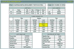
The controller proportional gains shown in the tuning are absolutely staggering. In over 15 years working in this field the author has never seen controller gains as high as this. It is pretty close to on/off control.
It is interesting to note how the tuning is derived by the Protuner. It is based on a full frequency response analysis derived mathematically from a step response and uses not only extremely sound mathematical principles, but also a 'tree of knowledge' laid out by one of the world's leading experts on loop optimisation. Typically in the 'loop signature' given in the bottom left hand side of the analysis report, one can see important information relating to the dynamics of the process. In this case the dead-time is 9,1 s and the dominant process time constant is 112 s. Where the dead-time is less than a tenth of the time constant the process tends to take on the characteristics of a pure lag process, wherein the phase lag never reaches -180°. Thus the loop cannot become unstable. This fact is taken into account in the tuning and the Protuner will give a more responsive tuning.
Initially, one's reaction to such a tuning is that it is crazy. However, there is seldom any harm in trying tuning to see how it works, and so a proportional gain of 45 and an integral of 1,5 min/repeat were inserted in the controller and a setpoint change made. The general expectation in the control room was that the loop would go wildly unstable. However, when placed in automatic, the tuning worked amazingly well and the response to a step change in setpoint was excellent. According to the process engineers this was the first time ever that the loop has worked properly in automatic. They were extremely impressed and very happy that a major control problem had been overcome. For interest’s sake the original 'as-found' tuning in the controller was a proportional gain of 1,1 and an integral of 0,5 min/repeat. Little wonder the control response was so slow.
In actual fact, even though the tuning gave excellent control, it would be very advisable to respan the pressure transmitter to a very much smaller span, in order to increase the process gain. This would allow the controller gain to be reduced. A high gain in a controller, although often necessary, does generally result in much more valve action and will tend to shorten the life of the mechanical equipment.


© Technews Publishing (Pty) Ltd | All Rights Reserved
 printer friendly version