


In the previous article in this series (www.instrumentation.co.za/16031r), it was shown that the main problem with the P-only controller is the fact that it is not capable of eliminating offset between the setpoint and process variable (PV) by itself. Manual reset was discussed, whereby the user can manually eliminate the offset by adjusting a bias added to the process demand (PD, the output signal from the controller). This, however, is a short-term solution, because another offset will arise if a load change occurs.
A mathematical genius in the 1930s found a simple way to overcome the offset problem, by introducing an automatic mechanism to eliminate offset. This is the I or ‘integral’ term.
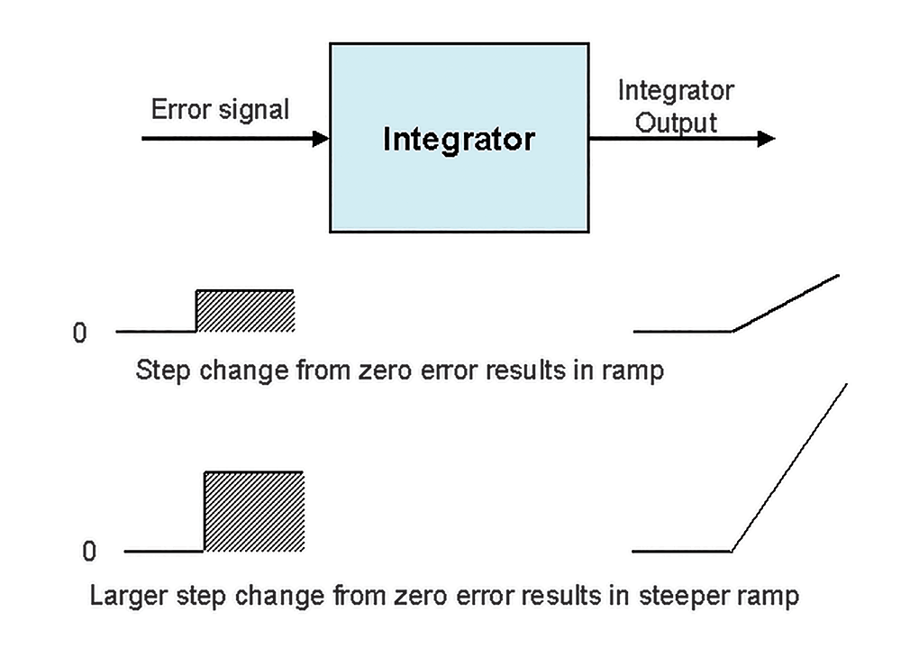 Figure 1. How an integrator works.
Figure 1 shows how an integrator works. The error signal is fed into the input of the device. If the error is zero, the output of the integrator remains fixed at whatever its current value is. However, if an error does appear at the input, then the unit starts integrating the error value with time. Thus, if the error input is a step, as shown in Figure 1, the output of the integrator will be a ramp, the slope of which will remain constant for as long as the error remains constant. If the error input is a larger step (bigger error) then the ramp will have a proportionally steeper slope. (It is important to note that the integral action in a controller is therefore greater the larger the error. Conversely, as the PV gets closer to setpoint, the integral ramp rate – and hence the effect on the PD – will be much less.)
The integrator acts as an automatic offset adjuster, because if any error arises on its input, it will try and move the output in a direction so as to diminish the error. As the error gets smaller, so too will the slope of the output ramp. When the error finally disappears, the integrator’s output will remain constant at its last value. Thus, it acts as an automatic bias to eliminate offset. It should be noted that the I term’s only purpose is to eliminate offset.
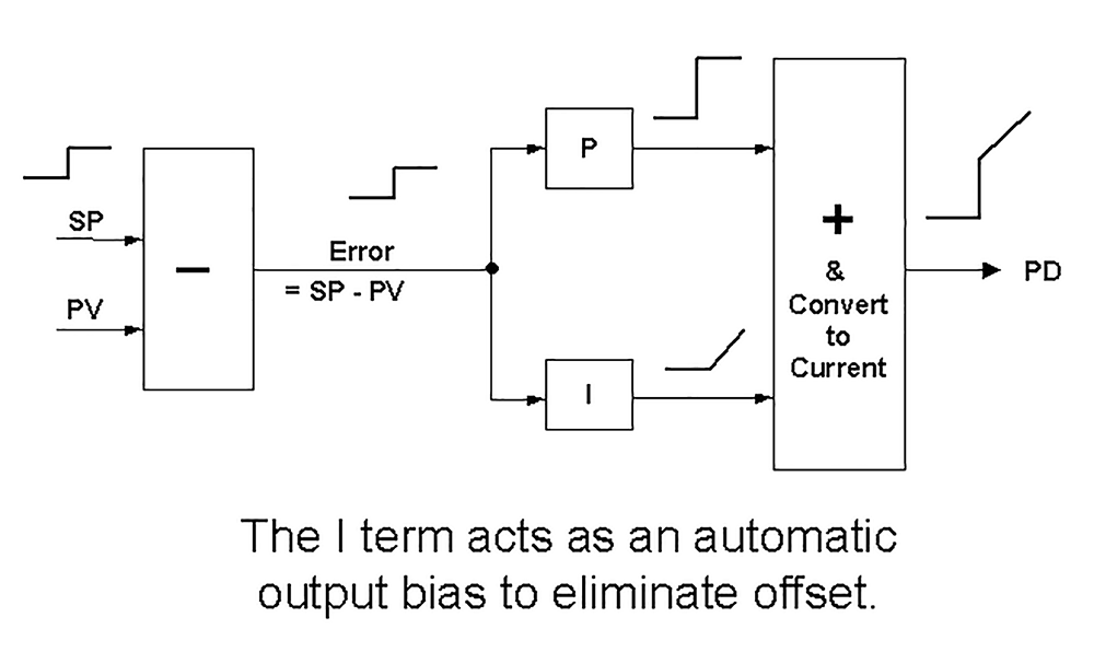 Figure 2. A simple P + I controller being tested.
Figure 2 illustrates a simple P + I controller which is being tested, as per the earlier article in this series (www.instrumentation.co.za/14984r) which covered controller test procedures. A setpoint step-change is made which results in a step change in error appearing at the input of both the P and I blocks. The output of the P block is a step, and the output of the I block is a ramp. The two responses are added as shown in Figure 2, so that the PD is a step followed immediately by a ramp.
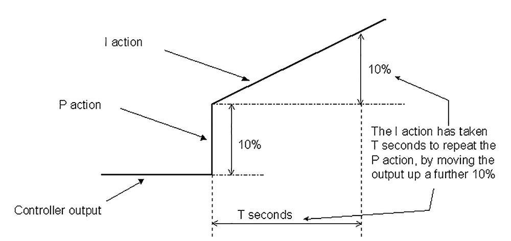 Figure 3. How the integral is measured on a series or ideal controller.
This response is dissected in Figure 3. Imagine that the step portion of the response, which is the contribution from the P block, has a magnitude of 10%. The I term then carries on increasing the PD at a constant ramp rate. If it takes, say, T seconds to raise the output a further 10%, it is said that the I term’s contribution has ‘repeated’ the P term’s contribution in T seconds.
The most commonly used units of measurement of the I term are seconds/repeat (or minutes/repeat) or the inverse, which is repeats/second (or repeats/minute). As usual, there are no standards, and each controller manufacturer uses whichever unit it wishes.
Note that these terms only apply to controllers with ‘series’ or ‘ideal’ algorithms. The time has now come to explain why the ‘parallel’ algorithm behaves so differently. In the aforementioned article on controller test procedures, it was mentioned that if one is to reduce the gain on controllers with series or ideal algorithms, the process response to a step change would be slower. Conversely, on a controller with the parallel algorithm, the response would become more cyclical.
The algorithm for the parallel controller with P + I tuning is:

The algorithms are the same for series or ideal controllers with P + I tuning (they differ only in the D term, if it is used):

It is important to note that in the latter algorithm, the P term also multiplies through into the I term, so if Kp is reduced, then the integral becomes slower, and the slope of the ramp is less.
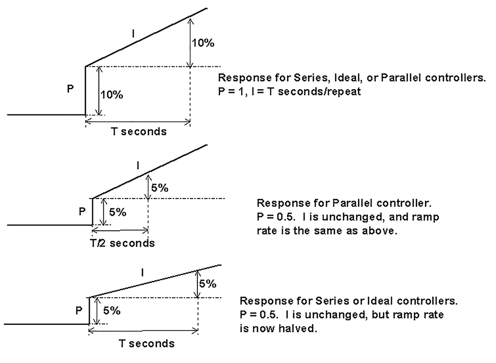 Figure 4. Response curves for different controller types.
The top graph in Figure 4 shows the response of a P + I controller undergoing testing. With the controller gain at Kp = 1, the I term is set to a value which, for both ideal and series controllers, would repeat the P action in T seconds. It should also be noted that a parallel controller would also have an identical response to this for Kp = 1, and with the same I value.
Now, in the parallel controller, if the gain were halved (Kp = 0,5) then nothing would happen to the integral ramp rate as the two terms are not linked at all. Therefore, on a 10% step change in error, the P action would result in an output step of 5%, and the integral would still continue ramping up at the same rate as it did in the previous test with Kp = 1.
This is shown in the middle graph in Figure 4. It is now observed that the P action is repeated in T/2 seconds. Therefore, the reason the parallel controller gets more cyclical when the gain is reduced, is because the integral effectively gets faster in relation to the P action.
In series and ideal controllers where Kp is multiplied with the I term, the integral ramp rate is now reduced by 50% and, as can be seen in the bottom graph in Figure 4, I repeats the P action in T seconds. Thus, the relationship between P and I is maintained.
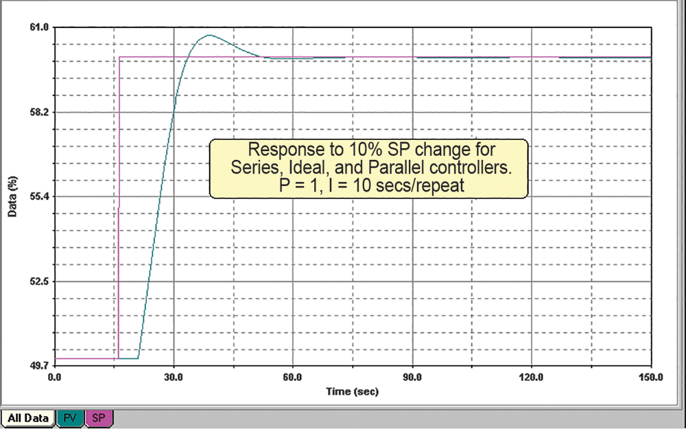
The difference between the closed-loop responses of series and parallel controllers controlling the same process with a reduction in the gain, but no change in integral, is shown in Figures 5, 6 and 7.
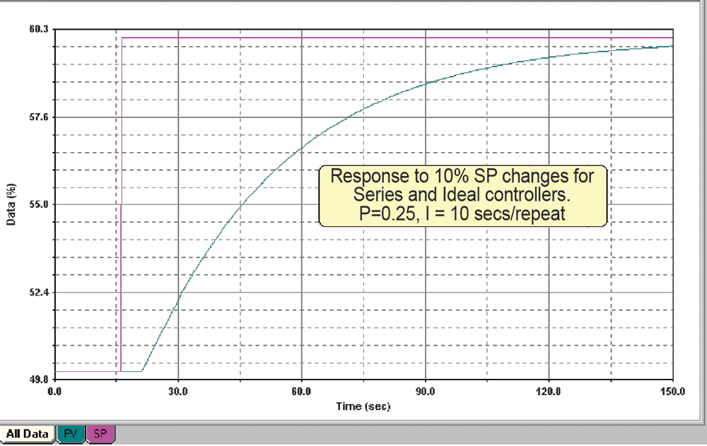 Figure 6. Response to 10% SP change for series and ideal controllers (P = 0,25, I = 10 sec/repeat).
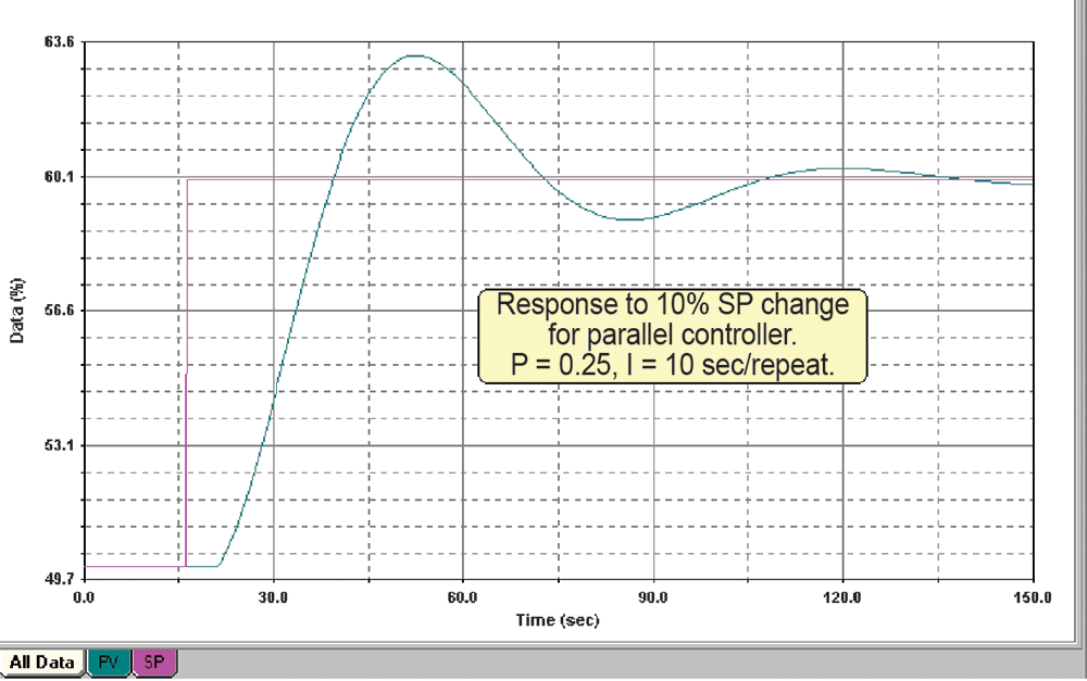 Figure 7. Response to 10% SP change for parallel controller (P = 0,25, I = 10 sec/repeat).
In Figure 5, the response for any of the three algorithms is the same, provided Kp = 1. In Figure 6, the response for the series or ideal controller is shown with Kp = 0,25, and the parallel controller in Figure 7, also with Kp = 0,25. Whereas the response on the former has become very slow, the latter has become much more cyclical. This means that if you were using the parallel algorithm and did indeed wish to reduce P by a factor of 4 to slow the response down, then you would also have to increase (lengthen) the integral by the same factor.
Thus, the parallel algorithm makes life extremely difficult for the poor instrument specialist, as tuning is made very much more complicated by having to adjust all the parameters simultaneously. Per the series or ideal algorithms on self-regulating processes, once you have the correct I (or I + D) settings, you can leave those terms alone and play only with the P ‘knob’ to obtain the desired response.
I have found that people who were wizards at tuning their plants when they worked on older controllers have lost their art completely when newer, computerised controllers were introduced which apply the parallel algorithm. This is because there is a completely different ‘feel’ to the tuning.
Fortunately, there was such resistance from users in the early days of computerised control systems using the parallel algorithm that manufacturers now generally offer the user a choice between parallel and at least one of the others. I would strongly recommend that you choose either the series or ideal algorithm – it will make your life very much easier when it comes to tuning.
At the time of writing this article I was doing some optimisation on a very remote diamond mine in southern Africa. The mine has standardised on a particular make of PLC for all its controls. Generally, as PLCs sometimes do not handle PIDs well, I always do some tests on them to check on the operation. In this mine we tested three PLCs – all of the same model – on different plants, and found that they were all reasonably accurate with the P action. However, they all had huge errors on the I timing response, ranging from –50% to +50% (the D response was not tested).
As the I function is completely time dependent, the problem obviously arises from the scan rate of how often the PID is executed in the PLC. Unfortunately, the manuals for the PLCs were really terrible with extremely poor, limited and confusing descriptions of the PID operation. Also, the plant personnel did not have any training on the PID operation, therefore it was impossible to say whether the problem was a manufacturing error or faulty programming.
The scan rate itself, as actually measured on the controller’s output, was very different to the setting in the controller’s program in the PLC, and did not tie in with any of the information given in the manual. The manual did, however, mention that the PID block should be executed in a sequence free from interrupts.
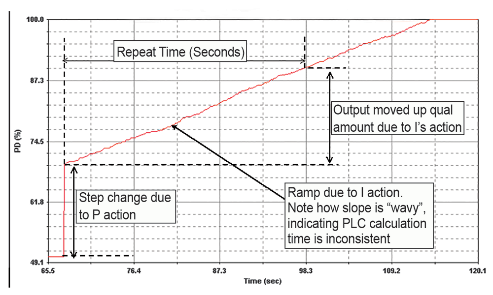 Figure 8. Results of controller testing on the PLC in a diamond mine.
Figure 8 shows one of the actual tests performed on the controller to check the P + I performance. It can also be seen in the test how the integral ramp is very ‘wavy’ which would indicate possible interrupts upsetting the PID timing execution.
The mine in question is now going to go back to the supplier to get help and more explanations on why the controllers are not performing properly, and why they are so far off specification.
About Michael Brown
 Michael Brown.
Michael Brown is a specialist in control loop optimisation, with many years of experience in process control instrumentation. His main activities are consulting and teaching practical control loop analysis and optimisation. He now presents courses and performs optimisation over the internet. His work has taken him to plants all over South Africa and also to other countries. He can be contacted at: Michael Brown Control Engineering CC,






© Technews Publishing (Pty) Ltd | All Rights Reserved
 printer friendly version