

In the previous two Loop Signature articles, several SWAG methods of tuning self-regulating processes were given. A very simple first-order lag deadtime process was tuned by those methods, and also by a couple of other methods including the Protuner, and the various responses to setpoint changes were shown. It was concluded that the reason that the SWAG tunings were all so different was because they were SWAG, and no such approximate method could ever give a really scientifically valid tune like the Protuner did.
Unfortunately, many plants have not invested in proper loop analytical and tuning equipment like the Protuner, and it is often extremely difficult to persuade management to commit to optimisation, as this means investment in time, people and equipment, all of which cost money. As mentioned in many of my articles in the Case History series, plants that have spent millions on a control system are often not prepared to invest a relatively small amount more to get their systems working properly, and in fact, in most cases have little idea how badly their investment in control is performing.
As a result, about 90% of all tuning performed work is done by WAG (wild ass guess) or ‘playing with the knobs’. Another 8% of people try SWAG methods, and the last 2% use truly scientific methods like the Protuner. The purpose of this particular article is to try and give those unfortunate enough to have to use WAG or SWAG tuning a bit of an idea of how to go about it and, even more importantly, some understanding of a couple of basic principles.
Unfortunately the methods discussed here will only work with really simple dynamics like a first-order lag deadtime self-regulating process. I cannot offer any advice on how to tune processes with a more complex dynamic without using the right equipment.
It is firstly necessary to know a little about the theory of tuning to understand how closed-loop control works. When you put a controller into automatic, you are actually performing a multiplication. Mathematically, the process and controller transfer functions are multiplied together. The best tuning, known as pole cancellation tuning, results in a combined transfer function, which is a perfect integrator.
This, out of interest, is exactly the same transfer function as an open-loop level process.
Pole cancellation tuning has major advantages, one of which is that it gives the lowest controller gain with the fastest integral, thus minimising valve wear and allowing fastest response to load changes. It was shown in Loop Signature 23 how a frequency plot was obtained by dynamic frequency testing. This involves applying a sine wave generator onto the process input or valve, and measuring the dynamic gain and phase shift at increasing frequencies until the PV lags the PD by 180°. The results can then be plotted on a frequency response graph, one of the most popular being the Bode plot, which was also shown in Loop Signature 23.
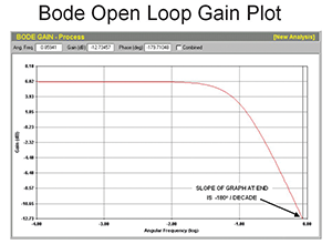
The Bode Gain plot of our simple first-order lag, self-regulating process is a graph starting off horizontally, and then dropping off to end at the point where the phase lag reaches -180°. An important point is that the slope of the gain plot at this point is –20d.b./decade (refer to Figure 1).
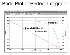
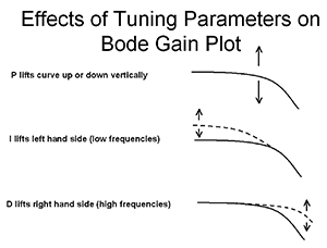
The Bode gain plot of a perfect integrator is shown in Figure 2. The gain plot is a perfectly straight line sloping downwards at exactly –20d.b./decade. This is the shape to which we must convert our simple first-order lag, self-regulating process, open-loop plot when it is multiplied by the controller’s transfer function. Now, in the controller we have only three terms to help achieve this. These are the P, the I and the D terms. Figure 3 shows the individual effect of each of these terms on the plot.
The P term has no effect on the shape of the plot. However, it does affect its position in relation to the Y axis (dynamic gain). The I term affects the lower frequencies section of the plot most. It tends to lift up the left-hand side. The D term has more effect on the higher frequencies section of the plot. It tends to lift up the right-hand side.
Now, the open-loop plot of our process already ends off at the right slope, so we can immediately see that we should never use the D term on such a process, as it will ‘mess up’ our pole cancellation. Therefore we are left to control this process with just the P and the I terms. As the P does nothing to the shape, it becomes obvious that the I term must do the work of straightening first, and then the P term will be used to set the response we require for the control.
A very interesting thing should be noted. If you refer to the last Loop Signature 25, where we tuned a simple process like this, you will see that the model we used had a time constant of 30 seconds. Then, in the tuning table you will see that the lambda tune gave an I value of 30,8 seconds/repeat, and both the IMC and Protuner gave an I value of 30,0 seconds/repeat.
It can be mathematically proved that if you set the I term equal to the time constant of a simple first-order self-regulating process, you cancel out the poles and get the perfectly straight line integrator closed-loop Bode plot we desire. This proof will be shown in a much later article, where the subject of process dynamics will be covered in detail.
Thus, the most important point of this article is that as far as self-regulating processes are concerned, once you get the combined plot straightened out as described, then you never again need to play with the I term, and in fact, also the D term if you did have to use it on more complex process dynamics.
Therefore, if I was unfortunate enough to have to ever tune a simple self-regulating process of this kind without a proper tuning package, I would use the following SWAG method:
• After ensuring that all the problems like valve hysteresis and non-linearity were sorted out, I would first do an open-loop step test on the process to allow me to determine the basic dynamics graphically, in particular the time constant (TC) and the dead-time (DT). All of these things were detailed in previous Loop Signature articles.
• If the DT<TC I would set the I term equal to the TC.
• If the DT>TC I would set the I term equal to the TC + Total loop DT/4. Total loop deadtime is the sum of the process deadtime and the controller scan rate.
• I would adjust P by trial and error to give me the response I may desire for that particular process. At any stage in the future, if I was not happy with that response, all I would have to do is play with the P term again. Provided the process dynamics had not changed, I would never again need to adjust the I.
This is very different from the way most people try to tune these types of processes with WAG. They generally always play with P first, and then try and adjust I. It’s much harder to do it that way.

About Michael Brown
Michael Brown is a specialist in control loop optimisation, with many years of experience in process control instrumentation. His main activities are consulting and teaching practical control loop analysis and optimisation. He now presents courses and performs optimisation over the internet. His work has taken him to plants all over South Africa and also to other countries. He can be contacted at: Michael Brown Control Engineering CC,
| Email: | [email protected] |
| www: | www.controlloop.co.za |
| Articles: | More information and articles about Michael Brown Control Engineering |


© Technews Publishing (Pty) Ltd | All Rights Reserved
 printer friendly version