In my last article, I wrote about how cascade control systems can effectively overcome valve problems. This article gives another example of how a temperature control was able to perform well, in spite of severe valve problems. The control in question used a cascaded secondary controller to control the flow of steam to a reboiler in a refinery. The temperature control was cycling, and we were requested to investigate this.
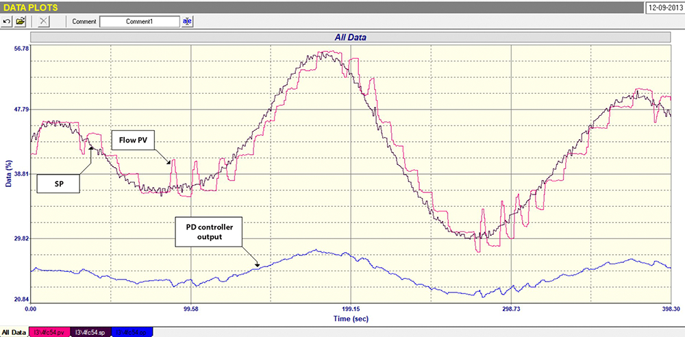
When analysing cascade controls one always starts with the secondary control loop, which in this case was the steam flow. Figure 1 is a closed loop ‘as found’ test, where one records the operation of the control in automatic prior to making any changes. In the recording one can see the operation of the flow with the controller’s set point in remote, i.e., it is connected to the output of the primary temperature controller. The first obvious thing that could be seen is that the set point was moving in a slow sinusoidal cycle.
To digress slightly, this was the problem which we had been requested to investigate and it was being caused by some external influence occurring on the column, and had nothing to do with problems in the actual temperature control. I will not be discussing this further in this article, but would just mention that the temperature control could not catch it, even with improved tuning, and it was decided that a further investigation needed to be carried out on the column to find out what was causing it.
The second thing that could be seen in the test was that the flow control was managing to keep the flow following the cycling set point fairly well, even though the flow seemed to jumping around quite badly and was itself cycling at times. However, these fluctuations would not have affected the actual temperature control as the temperature had much slower dynamics, which could not have reacted to the fluctuations as the correct average amount of heat would have been passed into the process.
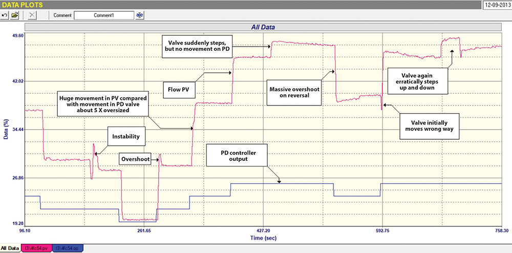
An open loop test was then carried out on the flow control. This is the main type of test that one needs to really analyse the components of the loop and determine if problems exist. This test is shown in Figure 2, and is really a remarkable example of illustrating some severe final control element problems:
One of the most striking things shown is that the valve is massively oversized, probably by about a factor of 5. This can be seen by looking at the ratio of the step sizes of PV to PD, which should ideally be about unity. As discussed in previous articles oversized valves ‘multiply’ all valve problems by the oversize factor including control variance.
The next obvious thing is that the control element does not follow the PD signal very well and jumps about in a very inconsistent fashion. Good examples of this are illustrated in the figure, some examples being:
• The PV on one occasion went into a small cycle.
• On some steps, but not all, the PV would overshoot by several percent and then come back.
• On one occasion, when the PD was constant, the PV suddenly stepped up by several percent and remained there.
• On another occasion it did the same thing, but this time only returned to its original value after about 30 seconds.
• On one step of the PD, the PV initially moved the wrong way.
At the operating conditions, the PD was working at about 20%, which is quite low. This is because of the huge valve oversizing. As a general rule, this is about the minimum where valves should be allowed to operate under normal control conditions. The reasons of this have been discussed in previous articles.
What can one conclude from these observations? Firstly, if good control is required, a five times oversized valve is very bad, and secondly, control would be affected badly with the valve performance being so erratic. Thirdly, one can easily conclude that there is a huge problem within the valve-positioner combination.
Just in passing, a very important point is that in many modern plants one can get a so called ‘valve position’ feedback signal directly fed back into the control room from the modern smart valve positioners. In many cases such as this, the signal may not reflect the problems that were seen in the open loop flow test, and it would give the erroneous impression that the positioner was doing a great job. The reason for this is that most of the positioners actually measure the position of the actuator stem, and not the true valve position. Therefore, in many cases where there are linkages or other things like gears between the actuator and the actual valve, problems are not seen.
What would the control have been like if they had not used the flow cascaded onto the temperature, and had rather placed the valve directly onto the PD of the temperature controller?
The answer is that there would probably have been no proper control with the valve in the condition that it was. The reason for this is that the temperature process had very slow dynamics, with a time constant in the order of several minutes. As discussed previously, a general fact is that one can only control slow processes slowly or instability can result. Therefore, if one was to use the fastest possible temperature controller parameters on the temperature controller, it would have taken a long time to try and get the valve to pass the correct amount of steam into the process, and by that time the valve may have jumped again, and it would be likely that one would never be able to get the temperature to the desired set point.
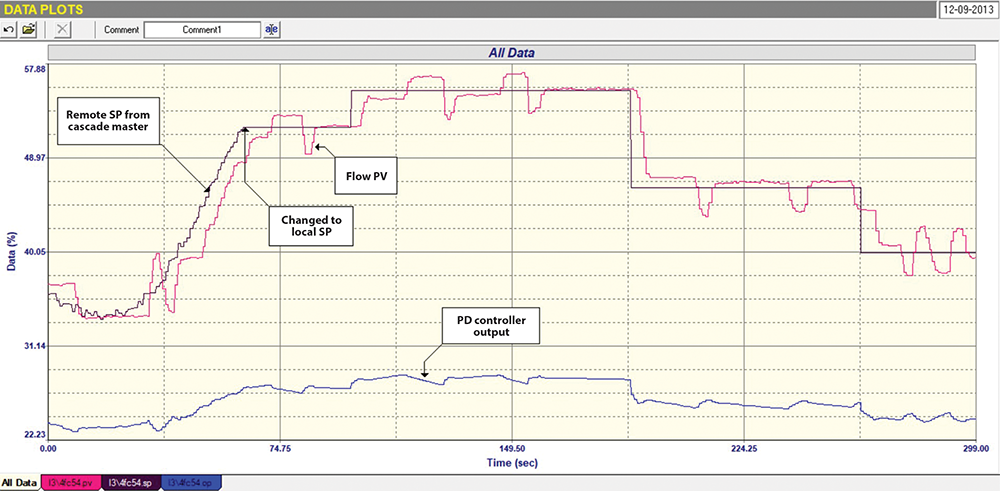
However, one could control the flow process very much faster as it had dynamics with time constants in the order of just a couple of seconds, and therefore could more or less keep the flow close to setpoint. Figure 3 shows a recording performed after both the temperature and flow loops had been properly tuned. One can see the flow loop running firstly in remote setpoint, and then in local setpoint to see how it performed with step changes.
When the set point was constant, the flow was pretty close to setpoint in spite of the valve jumping around badly at times. However, the average flow would certainly be good enough to satisfy the requirements of the temperature controller. The flow also reacted very well to even large setpoint step changes. When the setpoint was changing in part of the sinusoidal cycle, the flow did lag by a few seconds, but this would still be good enough for the temperature control.
It is another excellent example of the power of cascade control to overcome serious final control element problems.

About Michael Brown
Michael Brown is a retired specialist in control loop optimisation, with over 50 years of experience in process control instrumentation. His main activities were consulting and teaching practical control loop analysis and optimisation. He presented courses and optimised controls in numerous plants in many countries around the world. Michael is continuing to write articles based on the work he has done, and his courses are still available for purchase in .PDF format. He is still handling the sales of the Protuner Loop Optimisation software. He is happy to answer questions people may have on loop problems.
Contact details: Michael Brown Control Engineering CC,
| Email: | [email protected] |
| www: | www.controlloop.co.za |
| Articles: | More information and articles about Michael Brown Control Engineering |


© Technews Publishing (Pty) Ltd | All Rights Reserved
 printer friendly version