When analysing a control loop, one of the important things that one must do is to determine the dynamics of the process. Process dynamics can be loosely defined as various types of mathematical components that may be present in the response of a process to a change in the input. Industrial type processes may include one or more of the following dynamics: process gain, dead time, first and also higher order lags, multiple lags, and positive and negative leads.
Apart from gaining valuable information about the components in the control loop, it is essential to identify and possibly quantify these dynamic components in order to be able to tune the controller scientifically. In passing, it should be mentioned that the various dynamic components generally affect self-regulating processes differently from the way they do to integrating processes. This can make tuning of processes of complex dynamics very difficult, and it really becomes necessary for one to employ a good tuning package for these. Fortunately however, approximately 75 to 85% of all processes encountered in normal industrial process plants can be treated as having only two or more of the first three dynamics mentioned above, namely process gain, dead time, and a first order lag. These processes are relatively simple and in general if they can be identified properly, they can be tuned without the need for such a tuning package.
Ziegler and Nichols quickly realised in the 1930s that the ultimate method of tuning using dynamic operational testing which oscillates the process sinusoidally over a wide range of frequencies was not practical or feasible on industrial processes. They then pioneered research to establish other alternative methods for tuning. Although one of their methods was to use a limited cycle on the loop, and which works well on ideal loops, their other methods all involved making a mathematical model of the process by recording the response of the process to a step change on the input. One then graphically tries to determine the values of the two or three dynamics, and then plug the values into a formula to establish the tuning parameters. This is called ‘model based tuning’ and has not proved very successful, even though many other people have also come up with a variety of formulae. It works occasionally, but not often, and seldom gives really good tuning. However it can be adapted to serve with a certain amount of trial and error testing if you really understand what you are doing.
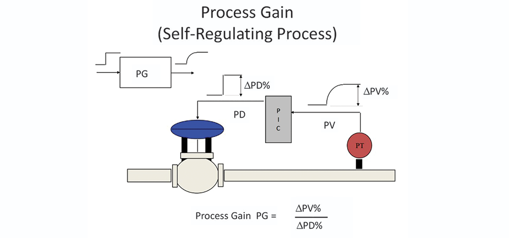
In this article we are going to discuss the process gain of a self-regulating process. Figure 1 shows how the PG (process gain) is measured for the response on a simple self-regulating process like a flow process. It is the ratio of the change in the PV (process variable) that results from a change in the PD (controller output). Note that it is best done by making a step change on the PD with the controller in manual.
The ideal value of PG is unity, as you are then making use of the full ranges of both the valve and the measurement. As a general rule, on a flow loop the PG is considered reasonable if it lies between 0,5 and 2. Problems can result if it is outside that range as described below. The value of the PG when measuring it on flow loops in particular can give valuable information as to whether the valve is oversized or if the transmitter span is too wide.
Oversized valves (PG>1) can cause two problems:
1. All valve problems are effectively multiplied by the PG value so that in closed loop control the control variance will be made worse by that value, and any cycling will cause the PV’s amplitude to be correspondingly that much bigger than the PD’s amplitude. For example if you have a stick-slip cycle occurring with the valve cycling over a range of say 2%, and the valve is four times oversized, then the amplitude of the cycle on the PV will be 8%.
2. Many fast self-regulating processes like fast flow loops are tuned with a very small proportional gain, and an extremely fast integral. For some unknown reason, some makes of controllers (even some very well known ones) have a very limited low end proportional gain setting. Typically, very commonly, it is limited to 0,1 (or 1,000% proportional band). I have even come across one make of PLC where the lowest value you can insert is 0,25. In many cases on these fast loops, and if the valve is oversized, then these controllers will not allow you to insert a small enough gain to prevent instability. To overcome this, one needs to increase the integral value, usually quite substantially. This adversely affects pole cancellation tuning, and can drastically slow down the tuning.
Transmitters with too wide a span (PG<1) also can cause two problems:
1. The accuracy and quality of the measurement can be badly affected. This is because you will always be working lower down on the measurement scale. Nearly all transmitters have a limited rangeability, with very few being able to give accurate or even valid measurements near the bottom of their range. (Also be aware that many types of transmitters have accuracies specified in terms of ‘% of full scale’, instead of ‘% of reading. This means that these transmitters are less accurate as you move down the scale.)
2. The PG is now small and must be less than unity. As the control speed of response to SP (setpoint) changes when in automatic is largely dependent on the product of PG (process gain) and Kp (controller gain) i.e. PG x Kp = Response, it means that as PG gets smaller you will have to put in a proportionally bigger Kp to get the desired response. Now, although it is sometimes necessary to use high Kp values to get the control response you need, what is happening here is that you are putting in a higher Kp than would be needed if you had a properly spanned transmitter. Remember, the higher the Kp, the more you are going to move the valve around, and this will result in a shorter valve life. I have come across quite a few cases where with very over-spanned transmitters, they have had to insert such a high Kp in the controller to get the desired speed of control response, and this has caused the controller’s output to fluctuate widely, with unacceptable valve movements. This is particularly the case where there is fairly high process noise on the PV. To overcome this, C&I; technicians or artisans often either drastically filter the PV, or else equally drastically reduce the Kp to ‘save the valve’. This means that one may not obtain the good control needed.
A brilliant example of this recently occurred when I was supervising loop bump tests on the controls of an offshore oil rig over the internet. The testing of the controls on this particular rig was very difficult due to the safety requirements. Any proposed test had to be first submitted to a panel for evaluation and approval with values given of size of steps etc. All the tests had to be performed by a senior operator and could not be done by the optimising team. This of course makes optimisation very slow and frustrating. However it is understandable as oil rigs are very hazardous plants, and safety is paramount.
The process in the example was a simple flow loop. The operators had been complaining that they had to run the loop in manual as it just didn’t seem to work properly in automatic. We first tried performing a closed loop test with the existing parameters where one makes a step change in SP. They would only allow a 9% change to be made. It was also initially found that they had the wrong controller setup on the controller, so that on SP changes there was only I (integral) action. They then changed this so that both P and I action came in. The result was that even after a few minutes it appeared as if the PV had not reacted.
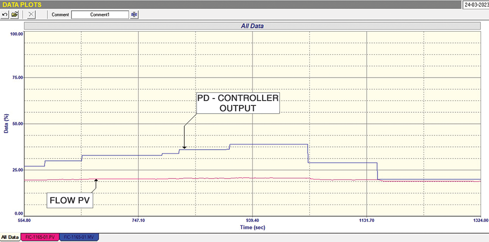
An open loop test was then performed, and this is shown in Figure 2. It should be noted that when performing these tests on our recording system we only see the variables trending on a 0-100% scale. The PD was moved up and down in a number of steps over a 20% range over a test lasting some 22 minutes. During this period there seemed to be no noticeable movement of the PV. It appeared to me that the valve was sticking. I wanted them to move the output further but the operators would not allow this as they thought that the valve might suddenly jump and cause a big surge in flow.
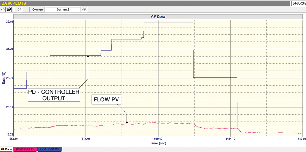
Later that day the C&I; staff on the rig emailed me the tests so I could examine them in more detail. On expanding the tests, to my amazement I saw that the flow was reacting to our changes fairly well but in tiny movements. The PG turned out to be an amazingly low 0,09. This is far too low and indicates there is something seriously wrong with the measurement scaling. The reason the process didn’t respond on the closed loop test was that their tuning was completely wrong, with a proportional gain some 40 times too low and an integral three times too slow.
It should also be pointed out that the flow was being measured using a differential pressure transmitter over an orifice plate. The flow was running below 20% of measurement, which is considered a region too low for this type of measurement. Generally the rule of thumb is that the measurement should be over 25%. However this did not really influence our observations.
This is a very interesting example of how measuring process gain can give you a big insight into loop problems.
Abourt Michael Brown

Michael Brown is a specialist in control loop optimisation, with many years of experience in process control instrumentation. His main activities are consulting and teaching practical control loop analysis and optimisation. He now presents courses and performs optimisation over the internet.
His work has taken him to plants all over South Africa and also to other countries. He can be contacted at: Michael Brown Control Engineering CC, +27 82 440 7790
| Email: | [email protected] |
| www: | www.controlloop.co.za |
| Articles: | More information and articles about Michael Brown Control Engineering |


© Technews Publishing (Pty) Ltd | All Rights Reserved
 printer friendly version