I was asked to investigate a problem of a drum pressure control that was cycling badly in a distillation column in a petrochemical refinery. The control team had spent a lot of time trying to stop the cycle by playing with the controller tuning. All to no avail.
Pressure control can fall into the class of either self-regulating processes or integrating processes. Here is a quick explanation for those not familiar with the two classes of processes. In self-regulating processes, when a step change is made on the input of the process, the output of the process moves to a new value and remains there. A typical example of self-regulating processes is a flow control.
An integrating process is a balancing process, where the output can only remain constant when the input and output are the same. If they are not equal, the output will always carry on changing. The best example of this is level control. For example if we wish to keep the level in a tank constant, then the outflow must be equal to the inflow. When the two are equal it is said that the process is in balance, and the value of the controller output (PD) is called the balance point.
These two classes of processes behave completely differently, and are also tuned completely differently. Unfortunately many instrument and control practitioners are not really aware of this, and may have little idea how to tune integrating processes.
In certain types of processes it can be very difficult to determine which class of process they fall into. Sometimes when there is a step change on the input, the process starts out behaving as integrating, and then after a while turns into a self-regulating process, or vice versa. A very good example of this is the level in a gravity-feed tank, where one relies on gravity for the outflow and there is no pump. The balance point value changes as the level varies. Other examples of this are encountered in many temperature control processes, and also in some pressure control processes in vessels containing compressible fluids like steam or gases.
In the example under discussion it was apparent that the pressure was behaving like an integrating process. To be able to perform both open and closed loop analytical tests on an integrating process it is essential to first stop the process cycling and get it balanced so that the process variable (PV) remains constant. This can often be difficult to do, particularly with very slow processes. One can try and do it by placing the controller into manual, and then trying to adjust the PD until it reaches a balance point and the cycling stops. However this can take an extremely long and often very frustrating time.
Without going into the reasons, a useful tip is that if integrating loops cycle in automatic then it is because of either of the following conditions:
• Hysteresis in the valve and with both proportional (P) and integral (I) control action set in the controller.
• Poor tuning, which is usually not too high a P gain, but normally is due to a poor setting of the I term, as few practitioners understand how to tune integrating processes properly.
Therefore to stop the cycling, one should try switching off the I term (and also the D term if it is set), and run the loop in
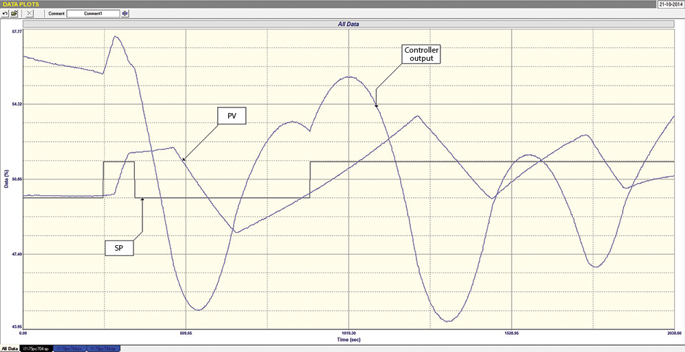
Once the process reaches a balance, one can perform the tests. Figure 1 is the As Found Closed Loop test on the process under discussion. The process had been brought fairly close to balance using the above procedure, and then the original tuning was reinserted into the controller and step changes were made in SP. The response of the PV is very interesting:
• On the first SP step, the PV seemed to stay where it was for 36 seconds. This could be due to a fairly long deadtime, or else the valve was not moving during this period.
• The PV then started rising quite swiftly, which immediately caused the PD to reverse direction, but this did not have any effect on the PV for a further 49 seconds. At this point one would have expected the PV to also start moving in a reverse direction, but it did not. It carried on ramping upwards for another 140 seconds, albeit at a much lower rate. This could indicate a severe valve problem.
• The PV then went into a slow cycle shaped like a sawtooth wave, whilst the PD cycled in a very sinusoidal fashion. This pattern on an integrating process is often an indication of severe valve hysteresis.
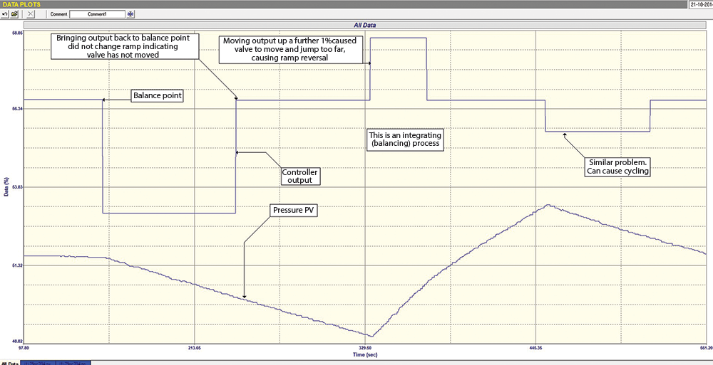
Figure 2 shows a portion of the Open Loop test. The controller is placed in manual when the process is in balance, and step changes are made on the PD. When a step change is made the PV will normally go into a constant ramp, which is the normal characteristic of a linear integrating process. One uses this response to perform scientific tuning.
On nearly all occasions, the PV responded to the step changes on the PD within two or three seconds, which is actually quite a short deadtime for an integrating process. This would again seem to confirm that the long deadtimes seen in the closed loop test were due to valve hysteresis, as opposed to a slow process deadtime or a sticky valve.
A very nice ramp was seen on the first step of PD. However on then stepping the PD back up to the balance point it was seen that the PD was still moving down at the same ramp rate. This shows that the valve had not moved, which is a further confirmation of valve hysteresis. Further steps of different magnitude of the PD in both directions showed that the hysteresis value was close to 4%. A general rule of thumb is that valve hysteresis should be less than 1%, and this gives a very clear picture of how badly hysteresis can affect a process, particularly an integrating process.
A new tuning was calculated and inserted in the controller. The original tuning was
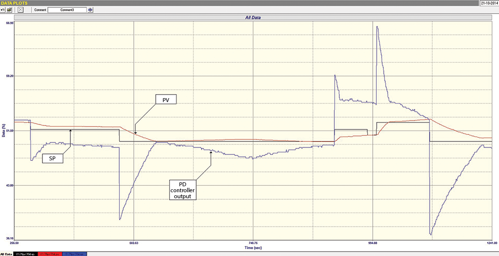
Figure 3 is the Final Closed Loop test with the new tuning. Although far from perfect, the control does operate a lot better. The instability is gone, however, the hysteresis on the valve is still creating difficulties for the controller to get the PV exactly to SP, as the PD still has to integrate through the hysteresis band of about 4% every time it tries to reverse the valve.
Once again, this is a wonderful example of how important it is for practitioners of optimisation to understand the practicalities of feedback control if they wish to successfully optimise a control loop.
About Michael Brown

Michael Brown is a specialist in control loop optimisation, with many years of experience in process control instrumentation. His main activities are consulting and teaching practical control loop analysis and optimisation. He now presents courses and performs optimisation over the internet. His work has taken him to plants all over South Africa and also to other countries. He can be contacted at: Michael Brown Control Engineering CC,
| Email: | [email protected] |
| www: | www.controlloop.co.za |
| Articles: | More information and articles about Michael Brown Control Engineering |


© Technews Publishing (Pty) Ltd | All Rights Reserved
 printer friendly version