The subject of noise has been covered in several recent articles in this series, and this is the last dealing with another aspect of this subject. It is a rewrite of a previous one that was published six years ago. I have done this, as I believe it is important that the subject should be included in the Loop Signature series.
When tuning noisy loops, we recommend in our courses that one should eliminate the noise by editing it out, so the tuning will be done only on the true process response, free of any noise. A delegate once asked me why this should be done. He argued that the controller does receive the signal with the noise in it, and surely the tuning should use the composite signal so that it can cope with the actual response complete with noise.
Our reply to this was that the controller is controlling the process, and is not controlling the noise. Therefore you must tune only on the process response.
This reply, although logical, does not really completely explain why you eliminate the noise. To really understand this matter one needs to understand the effect of disturbances coming into the loop at various frequencies.
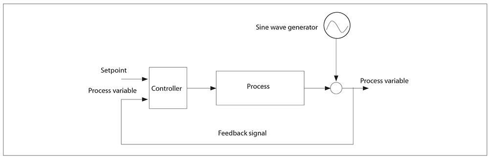
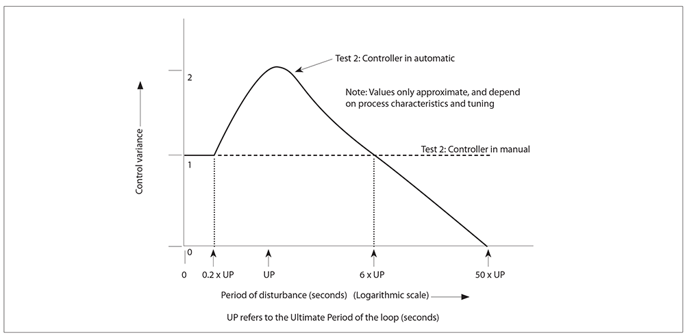
Figure 1 is the schematic of a control loop, where the disturbance in a sinusoidal signal is being injected into the PV signal. Figure 2 is a graph showing the results. The X-axis in Figure 2 represents the period of the sine wave. In other words, high frequencies start at the left-hand side of the graph and get slower towards the right. The value of the ultimate period of the loop is shown as UP on the X-axis. The ultimate period of a closed loop is the period of the continuous cycle which occurs in a closed loop when the gain in the controller (with only the P term in it) is turned up sufficiently to the point at which the loop becomes unstable. The frequency at which the cycle occurs, known as the ultimate cycle, can be thought of as the natural resonant frequency of the particular loop.
The Y-axis on the graph represents control variance. Control variance can be defined in various ways. However, when running statistical analysis of the control error, the variance may be defined as the standard deviation (σ) of the error. The paper industry usually uses 2xσ. For the purpose of this article, think of variance as the ‘quality of the control’.
In the first test, if the controller was placed into manual, and the variance measured over the frequency range, the loop could not respond to anything, because it was in manual. Therefore the variance would be constant over the whole range. Let us define the value of this variance as unity.
In the second test, the controller is in automatic, and the variance is plotted over the frequency range. It can be seen that at high frequencies there is no difference between the variance in manual or in automatic. This is understandable, as the control loop, and in particular the valve, cannot respond to high frequencies. However, as the period of the injected sine wave gets longer, a strange thing occurs. Instead of the controller starting to correct for the disturbance and improving the variance as might be expected, the variance starts getting worse.
This may make more sense when we realise that the closed loop has a natural resonant frequency of its own, and any external signal entering the loop with a frequency near the natural resonant frequency, will start ‘beating’ with the loop. The variance continues to increase as the period increases, until the period reaches a value somewhere between one and two ultimate periods. This is entirely dependent on the process characteristics and the type of tuning in the loop, which can alter the shape of the variance curve dramatically. The value of the variance reached can be as high as two. This means that the loop performance is twice as bad in automatic than in manual.
As the period of the disturbance increases even further, the variance then improves, until at roughly six to ten times ultimate period, the variance returns to unity. After that it keeps on improving, and finally, at somewhere between
People sometimes find this graph disturbing, because it is effectively telling us that feedback control cannot deal at all well with regular disturbances at frequencies near to the natural resonant frequency of the loop. The ultimate period of a typical liquid flow loop is about six seconds. This means that one would not really want regular disturbances entering the loop at periods between about one and 30 seconds, or else the controller will start reacting adversely to these disturbances, and in fact it would be better in manual than in automatic.
However, after some reflection we must realise that feedback control was never designed to deal with cyclical disturbances. It was designed to compensate for changes that occur on an intermittent basis. A good electrical analogy is that feedback was designed to operate on DC systems, not on AC systems. In fact, properly optimised feedback control generally does a brilliant job.
One can now understand quite a bit about feedback loop behaviour when faced with different type of disturbances. Firstly, the type of noise found on many fast regulating loops like noise are at high frequencies that lie well to the left of the peak of the curve. Provided these signals are not aliased into lower frequencies, as mentioned in an earlier Loop signature article, they will not affect the loop, and they can be ignored.
Lower frequencies that fall within the peak of the graph will cause increased variance and create problems. To deal with disturbances in this range, one should firstly try and eliminate them at their source. For example, better installation practices may help, like employing a stilling-well on level measurements, or using anti-aliasing filters on transmitters. If this cannot be done, then one may be forced to use a lag filter. As mentioned in a previous Loop signature article, filters are not desirable. In the case of very low frequencies, filters cannot be used, as they will completely kill the true process dynamics.
If all else fails, and provided the disturbances can be measured at their source, then feedforward decoupling is a powerful technique. It can operate very much faster than feedback control, and can be used to compensate for most cyclic load changes.
In many instances in plants suffering from cyclic load changes that cannot be eliminated at the source, one finds technicians and engineers spending frustrating hours trying to speed up the feedback tuning in a loop in a vain attempt to get it to control fast enough to deal with the changes. In actual fact, if the frequency of the disturbance is in the range of frequencies between
About Michael Brown
 Michael Brown.
Michael Brown is a specialist in control loop optimisation, with many years of experience in process control instrumentation. His main activities are consulting and teaching practical control loop analysis and optimisation. He now presents courses and performs optimisation over the internet. His work has taken him to plants all over South Africa and also to other countries. He can be contacted at: Michael Brown Control Engineering CC,
| Email: | [email protected] |
| www: | www.controlloop.co.za |
| Articles: | More information and articles about Michael Brown Control Engineering |


© Technews Publishing (Pty) Ltd | All Rights Reserved
 printer friendly version